How to Configure Your Redshift Cluster for Performance

Amazon Redshift is a popular cloud-based data warehousing solution that allows users to store and analyze large amounts of data quickly and efficiently. However, configuring a Redshift cluster for optimal performance can be challenging.

Here are the 5 key takeaways from this article:

• Properly selecting and configuring the type of Redshift node is crucial to achieving optimal performance. The author recommends starting with a dc2.large node and scaling up or down as necessary based on your workload.
• Redshift has several configuration settings that can be adjusted to optimize performance, including sort and distribution keys, compression encoding, and query optimization settings. Experimenting with these settings can significantly improve query performance.
• It's important to properly distribute data across nodes in a Redshift cluster. This involves selecting an appropriate distribution style for each table based on how the data will be queried and distributed keys.
• Redshift Spectrum, which allows you to query data stored in S3 as if it were in a Redshift table, can be a valuable tool for improving performance and reducing storage costs. However, it's important to properly configure your Spectrum tables and queries to avoid performance issues.
• Regular maintenance tasks, such as vacuuming and analyzing tables, are important for maintaining optimal Redshift performance. The author recommends setting up automated maintenance tasks to ensure these tasks are performed regularly.

In this article, we'll explore some best practices for configuring your Redshift cluster to achieve the best possible performance.

What’s the problem?

A frequent situation is that a cluster was set up as an experiment and then that set-up grew over time. Little initial thought went into figuring out how to set up the data architecture. Using best practices didn’t matter as much as moving fast to get a result.

And that approach is causing problems now. Lack of concurrency, slow queries, locked tables – you name it. But turns out these are not Redshift problems. They are configuration problems, which any cloud warehouse will encounter without careful planning.

The person who configured the original set-up may have left the company a long time ago. Somebody else is now in charge, e.g. a new hire. They inherit the set-up, often on short notice with little or no documentation. And now they face the task of re-configuring the cluster.

Setting up your Redshift cluster the right way

We call that “The Second Set-up” – reconfiguring a cluster the right way, and ironing out all the kinks.

The upside is huge. High scalability and concurrency, more efficient use of the cluster, and more control. No more slow queries, no more struggling with data, lower cost.

So in this post, I’m describing the best practices we recommend to set up your Amazon Redshift cluster. It’s also the approach we use to run our own internal fleet of over ten clusters. And it’s also the approach you can – and should! – use when you’re setting up your cluster for the first time.

Unlike other blog posts, this post is not a step-by-step instruction of what to do in the console to spin up a new Redshift database. You can read the documentation for that. Instead, we cover the things to consider when planning your data architecture. That’s an important distinction other posts fail to explain.

So let’s start with a few key concepts and terminology you need to understand when using Amazon Redshift. And then we’ll dive into the actual configuration.

1. Glossary of terms

Cluster: A “cluster” is a collection of “nodes” which perform the actual storing and processing of data. Each cluster runs an Amazon Redshift engine.

Nodes: AWS offers four different node types for Redshift. Each node type comes with a combination of computing resources (CPU, memory, storage, and I/O). Pricing for Redshift is based on the node type and the number of nodes running in your cluster. By adding nodes, a cluster gets more processing power and storage.

Database: A cluster can have one or more databases. A database contains one or more named schemas, which in turn contain a set of tables and other objects.

Schema: A schema is the highest level of abstraction for file storage. Schemas organize database objects into logical groups, like directories in an operating system.

Queues: Redshift operates in a queuing model. When a user runs a query, Redshift routes each query to a queue. Each queue gets a percentage of the cluster’s total memory, distributed across “slots”. You can define queues, slots, and memory in the workload manager (“WLM”) in the Redshift console. By default, an Amazon Redshift cluster comes with one queue and five slots. Queues and the WLM are the most important concepts for achieving high concurrency. I write about the process of finding the right WLM configuration in more detail in “4 Simple Steps To Set-up Your WLM in Amazon Redshift For Better Workload Scalability” and our experience with Auto WLM.

Superuser: A superuser has admin rights to a cluster and bypasses all permission checks.

User: A single user with a login and password who can connect to a Redshift cluster.

User Groups: A group of users with identical privileges. Any change to the access rights of a user group applies to all members in that group.

Data Apps: Applications for your ETL, workflows, and dashboards. Data apps are a particular type of user. They have a single login to a cluster, but with many users attached to the app.

IAM policy: An IAM policy defines the permissions of the user or user group. AWS offers a set of pre-defined IAM policies for Redshift. 

These are the key concepts to understand if you want to configure and run a cluster. Now let’s look at how to orchestrate all these pieces.

2. Why you shouldn’t use the default cluster configuration

Let’s start with what NOT to do – and that’s using the default configuration for a cluster, which is:

• one schema (‘public’)
• one user (‘masteruser’, which is a superuser)
• one WLM queue (‘default’) with five slots

It may be counter-intuitive, but using the default configuration is what will get you in trouble.

At first, using the default configuration will work, and you can scale by adding more nodes. But once you’re anywhere between 4-8 nodes, you’ll notice that an increase in nodes doesn’t result in a linear increase in concurrency and performance.

Common issues you will encounter are slow or hanging queries, table locks, and lack of concurrency. I’m covering the issues from using the default configuration more in “3 Things to Avoid When Setting Up an Amazon Redshift Cluster“.

You need to configure your cluster for your workloads. And here, Redshift is no different than other warehouses. If you misconfigure your database, you will run into bottlenecks. And so it’s a myth and misconception that Redshift doesn’t scale. As we’ll see, it’s quite the opposite.

What is true about Redshift is that it has a fair number of knobs and options to configure your cluster. That may seem daunting at first, but there’s a structure and method to use them. Once you have that down, you’ll see that Redshift is extremely powerful.

So let’s look at how to do it right.

3. The Recommended Setup for your Redshift Cluster

When approaching the set-up, think about your Redshift cluster as a data pipeline. The pipeline transforms data from its raw format, coming from an S3 bucket, into an output consumable by your end-users. The transformation steps in-between involve joining different data sets.

One Cluster with one IAM Policy

Amazon Redshift supports identity-based policies (IAM policies). We recommend using IAM identities (e.g. a user, a group, a role) to manage cluster access for users vs. creating direct logins in your cluster. That’s because nobody ever keeps track of those logins.

When using IAM, the URL (“cluster connection string”) for your cluster will look like this:

jdbc:redshift:iam://cluster-name:region/dbname

You can find your cluster connection string in the Redshift console, in the configuration tab for your cluster. Please see the Redshift docs for downloading a JDBC driver to configure your connection.

By using IAM, you can control who is active in the cluster, manage your user base and enforce permissions. You’re running your cluster within the security policies of your company.

Using IAM is not a must-have for running a cluster. We do recommend using it from the start as it makes user management easier and secure. That may not seem important in the beginning when you have 1-2 users. But it will help you stay in control as your company and Redshift usage grows. For example, we use IAM to generate temporary passwords for our clusters.

Your Redshift cluster only needs one database

1. prod

dev is the default database assigned by AWS when launching a cluster. You can rename that db to something else, e.g. “prod”.

It’s possible to run more than one database in a cluster. But we recommend keeping it simple – one cluster, one database.

Databases in the same cluster do affect each other’s performance. For example, you have “dev” and “prod”. You’re loading a large chunk of test data into dev, then running an expensive set of queries against it. These queries are using resources that are shared between the cluster’s databases, so doing work against one database will detract from resources available to the other, and will impact cluster performance.

In Amazon Redshift, you cannot run queries across two databases within a cluster. To do so, you need to unload/copy the data into a single database.

Your Redshift cluster should have Two Schemas: raw and data

1. raw schema

The ‘raw’ schema is your staging area and contains your raw data. It’s where you load and extract data from. Only data engineers in charge of building pipelines should have access to this area.

2. data schema

The “data” schema contains tables and views derived from the raw data. Analysts can query and schedule reports from this schema. Depending on permissions, end-users can also create their own tables and views in this schema.

The separation of concerns between raw and derived data is a fundamental concept for running your warehouse.

The raw schema is your abstraction layer – you use it to land your data from S3, clean and denormalize it and enforce data access permissions. From there, you can model and create new datasets you expose in the “data” schema.

Downstream users like data scientists and dashboard tools under no circumstance can access data in the raw schema. The moment you allow your analysts to run queries and run reports on tables in the “raw” schema, you’re locked in. You can’t remove that table anymore without breaking the downstream queries.

Multi-schema set-up

Of course, you’re not limited to two schemas. The point here is to maintain the abstraction between raw and derived data in your schemas. You can set up more schemas depending on your business logic.

For example, some of our customers have multi-country operations. They use one schema per country. The corresponding view resembles a layered cake, and you can double-click your way through the different schemas, with a per-country view of your tables.

Tracking schema growth

Another benefit of abstracting your data architecture at the schema level is that you can track where data growth is coming from. That’s helpful when e.g. when your cluster is about to fill up and run out of space.

With intermix.io, you can track the growth of your data by schema, down to the single table. Below you can see how a spike in cluster utilization is due to a growth of the “public” schema. From there, you can double-click on the schema to understand which table(s) and queries are driving that growth.

Additional schema settings and operations

Once you’ve defined your business logic and your schemas, you can start addressing your tables within the schemas. We’re covering the major best practices in detail in our post “Top 14 Performance Tuning Techniques for Amazon Redshift”.

For the purpose of this post, there are three key configurations and operations for your tables to pay attention to:

1. Choose a DIST KEY, a table property that decides how to distribute rows for a given table across the nodes in your cluster. Choosing the correct distribution style is important for query performance. A wrong distribution style causes “row skew” or “data skew”, resulting in uneven node disk utilization and slower queries.
2. Pick a SORT KEY to determine the order to store the rows in a table. With the right Sort Key, queries execute faster, like planning, optimizing and execution of a query can skip unnecessary rows. The lower your percentage of unsorted rows in a table, the faster queries your queries will run.
3. Run VACUUM on a regular basis to keep your “stats_off” metric low. Vacuuming is a process that sorts tables and reclaims unused disk blocks. A lack of regular vacuum maintenance is the number one enemy for query performance – it will slow down your ETL jobs, workflows, and analytical queries.

In Integrate.io, you can see these metrics in aggregate for your cluster, and also on a per-table basis.

Your Cluster Should Have Four User Categories

1. Superuser Category

When spinning up a new cluster, you create a master user, which is a superuser. A superuser bypasses all permission checks and has access to all schemas and tables.

Limit the number of superusers and restrict the queries they run to administrational queries, like CREATE, ALTER, and GRANT. A superuser should never run any actual analytical queries.

2. Load User Category

Users that load data into the cluster are also called “ETL” or “ELT”. Users in the “load” category write to the “raw” schema and its tables.

Load users run COPY and UNLOAD statements.

Common applications for “ETL” are Stitch, Segment, Fivetran, Alooma, Matillion, and ETLeap. integrate.io is also in this category, as we run the UNLOAD command to access your Redshift system tables.

3. Transform User Category

Scheduled jobs that run workflows to transform your raw data. Users in the “Transform” category read from the “raw” schema and write to the “data” schema.

Transform users run INSERT, UPDATE, and DELETE transactions.

Popular schedulers include Luigi, Pinball, and Apache Airflow. By far the most popular option is Airflow. If you don’t want to run Airflow yourself, companies like Astronomer.io offer hosted versions.

4. Ad-hoc User Category

Queries by your analysts and your business intelligence and reporting tools.

Ad-hoc users run “interactive” queries with SELECT statements.

Popular business intelligence products include Looker, Mode Analytics, Periscope Data, and Tableau. Also in this category are various SQL clients and tools data scientists use, like datagrip or Python Notebooks.

If you’re unclear what type of commands your users are running, in integrate.io you can select your users and groups, and filter for the different SQL statements/operations. It’s a fast and intuitive way to understand if a user is running operations they SHOULD NOT be running.

Those 4 User Categories Should Fit into Three User Groups

1. Loads

All users in the “load” category.

2. Transforms

All users in the “transform” category.

3. Ad-hoc

All users in the “ad-hoc” category.

By using Groups, you separate your workloads from each other. Groups also help you define more granular access rights on a group level.

Like with schemas, you can create more granular user groups, e.g. to reflect lines of business or teams. For example, you can create user groups by business function, e.g. ‘finance’, ‘analysts’, or ‘sales’. With more granular groups, you can also define more granular access rights. We do recommend that approach, as long as you maintain the separation of concerns by workload type.

Your Cluster Needs Four WLM Queues

1. Load

Assign the “load” user group to this queue.

2. Transform

Assign the “transform” user group to this queue.

3. Ad-hoc

Assign the “ad-hoc” user group to this queue.

4. Default

No users are assigned apart from select admin users.

We learned in the “Key Concepts” section that Redshift operates in a queuing model. The default setting for a cluster is a single queue (“default”) with a concurrency of five.

With the three additional queues next to “default”, you can now route your user groups to the corresponding queue, by assigning them to a queue in the WLM console. Because of Redshift’s queuing model, any user that is not part of a group gets routed to the default queue.

Queues are the key concept for separating your workloads and efficient resource allocation. You will see that similar workloads have similar consumption patterns. In general:

• “Load” queries are low memory and predictable.
• “Transform” queries are high memory and predictable
• “Ad-hoc” queries are high memory and unpredictable.

By routing these queries to corresponding queues, you can find the most efficient memory/slot combination. You’re also protecting your workloads from each other. For example, a long-running ad-hoc query won’t block a short-running load query as they are running in separate queues.

For more detail on how to configure your queues. please read my post 4 Simple Steps To Set-up Your WLM in Amazon Redshift For Better Workload Scalability

Activate additional WLM settings

There are three additional WLM settings we recommend using.

1. Activate “Short Query Acceleration” in your WLM console. SQA prioritizes the execution of smaller, short-running queries.
2. Enable “Concurrency Scaling”, to handle peak loads for your ad-hoc queries. With Concurrency Scaling, Redshift adds additional cluster capacity on an as-needed basis, to process an increase in concurrent read queries.
3. Define WLM Query Monitoring Rules to put performance boundaries for your queries in place. For example, you can create rules to abort queries in your ad-hoc queue that run longer than e.g. 10 minutes.  

Using both SQA and Concurrency Scaling will lead to faster query execution within your cluster. With WLM query monitoring rules, you can ensure that expensive queries caused by e.g. poor SQL statements don’t consume excessive resources.

Summary & Configuration

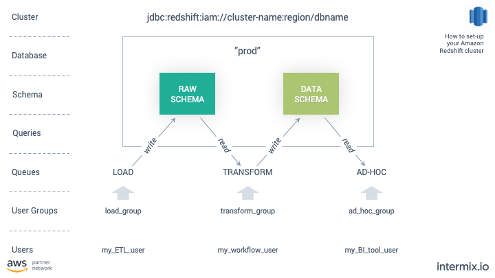
So let’s put this all together:

• 1 cluster: jdbc:redshift:iam://cluster-name:region/dbname

• 1 database: prod

• 2 schemas: raw, data

• 4 user categories: superuser, load, transform, ad-hoc

• 3 user groups: load, transform, ad–hoc

• 4 queues: load, transform, ad-hoc, default

A picture tells a thousand words, so I’ve summarized everything into one chart.

The work related to the set-up  – creating the users and groups, assigning them to queues, etc. – takes about one hour.

The result is that you’re now in control. Knowing the cluster as a whole is healthy allows you to drill down and focus performance-tuning at the query level. On that note – have you looked at our query recommendations?

Cost-Performance Benefits of this Cluster Configuration

Beyond control and the ability to fine-tune, the proposed set-up delivers major performance and cost benefits. We’ve found that a cluster with the correct setup runs faster queries at a lower cost than other major cloud warehouses such as Snowflake and BigQuery.

In their report “Data Warehouse in the Cloud Benchmark”, GigaOM Research concluded that Snowflake is 2-3x more expensive than Redshift. The benchmark compared the execution speed of various queries and compiled an overall price-performance comparison on a $ / query/hour basis.

Conclusion

With the right configuration, combined with Amazon Redshift’s low pricing, your cluster will run faster and at a lower cost than any other warehouse out there, including Snowflake and BigQuery.

The challenge is to reconfigure an existing production cluster where you may have little to no visibility into your workloads. By adding Integrate.io to your set-up, you get a granular view into everything that touches your data, and what’s causing contention and bottlenecks. You can focus on optimizing individual queries,

The Unified Stack for Modern Data Teams

Get a personalized platform demo & 30-minute Q&A session with a Solution Engineer

GET A LIVE DEMO